
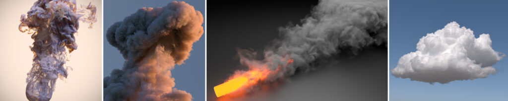
Course NPGR010 (2026/2027)
| Lectures: | Wednesdays, 15:40 – 17:10, room S5 | Contact: Tomáš Iser |
| Practicals: | Thursdays, 15:40 – 17:10, room SU2 | Contact: Tomáš Iser |
Please note: Be cautious when looking at the archived materials from previous years. Some of the slides and assignments are different.
Course grading
The course consists of “zápočet” (credit from labs) and a final exam.
To pass the labs, the student must submit correct solutions to five (5) assignments and actively participate in the labs at least five times (5x). An active participation includes solving a problem at the blackboard, presentation of the first assignment (3D scene), correctly answering in mini-exams, etc. The student has the right to repeat some of these attempts according to the study rules.
To pass the final exam, the student has to receive at least 55% points from the exam.
The final grade is determined by the points from the exam.
Lecture content
Slides and course notes will be updated troughout the semester.
Date |
Topic |
Slides & Notes |
| 30 September | Introduction to the course Basic explanation of terminology such as rasterization, ray casting, ray tracing, path tracing, ray marching, meshes, solids, surfaces, volumes, signed distance fields, shading, etc. |
Slides |
| 7 October | Reflection equation and radiometry Photon model and wave model, power (flux), radiant intensity, irradiance, radiance, inverse square law, Lambert’s cosine law |
|
| 14 October | Numerical integration Numerical quadrature, Monte Carlo, properties of a Monte Carlo estimator, random sampling |
|
| 21 October | Monte Carlo in rendering and importance sampling Using Monte Carlo in ray tracing, random sampling, importance sampling; example of importance sampling a diffuse and specular lobe of a BRDF |
|
| canceled (bank holiday) | ||
| 4 November | Monte Carlo in rendering and importance sampling — continued Importance sampling an environment map and area lights; a bit on control variates and stratification Multiple importance sampling (MIS) Motivation of MIS, formula, balance heuristic, example with BRDF/envmap |
|
| 11 November | Multiple importance sampling (MIS) — continued Example with BRDF/area lights, examples of other heuristics (cutoff, power, maximum) Building a path tracer Constructing the rendering equation, the operator form, Neumann series, recursion, implementation with a for loop with maxLength (fixed path length → bias) |
|
| 18 November | Building a path tracer — continued Implementation with a while loop (using Russian roulette → unbiased), the principles of: 1) adjoint-driven Russian roulette & splitting, 2) path guiding, 3) next event estimation (NEE), NEE with multiple light sources (“many-light methods”) |
|
| 25 November | Volumetric light transport and participating media Surface vs. volume rendering, examples of participating media, Beer-Lambert law including derivation, volume rendering equation (VRE) including derivation, distance sampling in a homogeneous volume proportional to transmittance (including derivation), basics of distance sampling in heterogeneous volumes (main principles of regular tracking, ray marching, and null-collision algorithms) |
|
| 2 December | Bidirectional path tracing (BDPT), photon mapping (PM) Only the main principles without going too deep into technical details BDPT: Measurement equation, duality of importance and radiance, path tracing vs. light tracing, path integral formulation, constructing paths in bi-directional path tracing and using MIS (no derivations) PM: Problem of SDS paths, photon tracing (including formulas), photon maps, rendering with photon maps (caustics vs. final gathering) Any additional information in the slides that is not mentioned above will not be examined |
|
| 9 December | Inverse and differentiable rendering Only the main principles without going too deep into technical details Inverse problems, various ways to find the optimum, gradient descent, finite differences, automatic differentiation (AD), forward-mode AD, reverse-mode AD, situations that cause problems (ambiguities, discontinuities) |
|
| 16 December | Neural fields and Gaussian splatting Only the main principles without going too deep into technical details |
|
| 6 January | Denoising |
Practicals / labs content
Date |
Topic |
Slides & Notes |
| 1 October | Introduction to Blender Homework assignment 1 Math exercises (radiometry): solid angle, spherical coordinate system, integrals in spherical coordinates, differential solid angle, differential area |
|
| 8 October | Introduction to random sampling Math exercises: expected value, variance, probability distribution function, cumulative distribution function, normalization, random sampling in 1D, multidimensional random sampling |
|
| 15 October | Assignment 1 deadline + student presentations (5-8 minutes / student) | |
| 22 October | Homework assignment 2.1 “Ray tracing with light source sampling” | |
| 29 October | Consultation | |
| 5 November | Assignment 2.1 deadline Homework assignment 2.2 “Ray tracing with BRDF sampling” |
|
| 12 November | Consultation | |
| 19 November | Assignment 2.2 deadline Homework assignment 2.3 “Ray tracing with multiple importance sampling (MIS)” |
|
| 26 November | Consultation | |
| 3 December | Assignment 2.3 deadline Homework assignment 2.4 “Path tracing” |
|
| 10 December | Consultation | |
| 17 December | Assignment 2.4 deadline | |
| 7 January | First examination date (“předtermín”) |
Math exercises
Below, you can find a handful of pen & paper exercises that are useful when studying light transport. We will cover some of these during the labs.
Spherical integrals
- What is the difference between an angle and solid angle, between radians and steradians?
- What is the meaning of x radian on a unit circle, and x steradian on a unit sphere?
- What are spherical coordinates? Derive the conversion from Cartesian to spherical coordinates, and vice versa.
- What is the solid angle under which we observe an (infinite) plane from a point outside of the plane?
- How do you transform a spherical integral ∫ f(ω) dω to a double integral ∫∫ _____ dθ dφ ? What are the bounds and missing term(s)?
- Derive that the surface area of a unit sphere is 4π using the spherical integral above.
- Similar exercises (hint: just change the bounds of the above integral):
- Calculate the surface area of a spherical cap delimited by the angle α measured from the north pole.
- Calculate the surface area of a spherical wedge with angle β.
- Calculate the solid angle under which we observe a sphere with radius R, the center of which is at the distance D from the observer.
Assignment 1 (“Creative exercise”)
Deadline: 15 October 2026 15:40
In this course, we focus on writing algorithms for photorealistic rendering. But what use is it to know an algorithm if you cannot even create your own 3D scene? That is why our first assignment is and has traditionally been to create and render a 3D scene.
If you are not familiar with any 3D editing and rendering software, I recommend to use Blender, which is free and comes with a built-in path tracer called Cycles. Students can use any other 3D editing software (e.g., Autodesk 3ds Max) and any other renderer which uses path tracing (e.g., Autodesk Arnold). Please do not use renderers that are primarily based on rasterization, such as Unreal or Unity.
Your goal is to create and render a 3D scene and satisfy the following requirements:
- The scene must use at least 6 very different materials
(e.g., glass, plastic, wood, concrete, liquid, fabric, metal) - At least one of the materials must have subsurface scattering
- The scene must use at least the following light sources:
- Environment map / HDRI
- Area light (e.g., a rectangle)
- You have to render the scene multiple times, split into the following components:
- Direct vs. indirect illumination
- Diffuse vs. specular (or glossy) reflections
- You must demonstrate the use of denoising:
- Render the scene once without denoising, with a very low sample count to get a noisy render
- Render the scene once without denoising, with a very high sample count to get a smooth, converged render
- Render the scene once with a very low sample count and with denoising enabled
Prepare a presentation (5-8 minutes) with the images and describe what we can see on them. Also explain your motivation behind the scene that you modeled.
You can use free resources that you download on the internet, such as textures, environment maps, meshes, and so on. You cannot download the entire scene though as the point of the exercise is for you to try to at least insert and transform the objects into a scene, apply materials on them, position a camera, etc.
This is an individual exercise and you should not work in a team.
Assignments 2.1 – 2.4 (“Programming exercises”)
Will be explained later.
Archive
Course information for the previous academic years: